Project 1

First Steps

I used the zillow_scrape.py file provided in class to scrape 400 listings from Zillow for houses for sale in Detroit, MI. I chose Detroit because I am moving to Michigan next year and wanted to learn about the housing market there. The output file exported the data as a .csv file which I then imported into a different python file for data processing.

Data Description

• The output file had the variables of listing price, number of bedrooms, number of bathrooms, square footage, and address.
• 16 of the listings did not have number of bedrooms and bathrooms listed (null values), so I dropped those listings
• 8 of the listings did not have square footage listed. I ran the model to see if it would impute values for square footage, but instead the model did not perform and only had NaN values for the loss. I dropped those 8 listings as well.
• I decided that one of the variables I wanted to consider in the model was location, so I used geopy to convert addresses to latitude, longitude, and altitude. This website was very helpful: Geocode with Python.
  • Some of the address values in the conversion could not be recognized and converted to a latitude and longitude. The output made those listings have NaN values for the latitude/longitude, so I dropped those values as well. There were 68 of those, so I knew that by dropping them, I was potentially making my model less accurate. I decided that having a location variable was more worth it than having 400 data points for running the model.

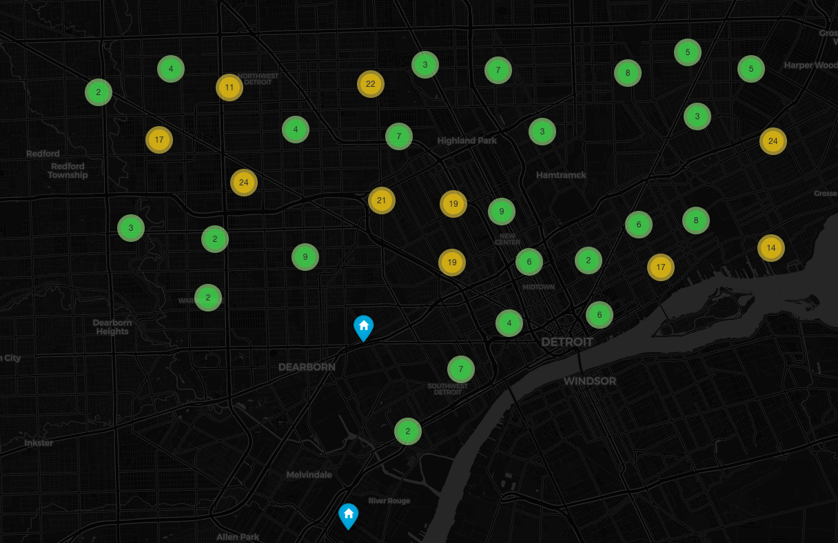
Figure 1. Mapped Addresses using converted latitude and longitude

I created a webmap for all of the addresses, but I couldn’t figure out how to host a .html file on github, so here’s a screenshot of the web map. The homes are grouped and when you zoom in on the map, it shows you the homes for sale.

Data Summary

Variable	Max	Min	Mean
Price ($)	2,200,000	1,000	146,000
Number of Bedrooms	7	2	2.5
Number of Baths	1	7	2.5
Square Footage (ft^2)	7075	770	2041

Model Architecture

The model I used is the same one that we used for identifying the Matthews, VA house prices. Because I decided to use location as an additional variable, I have 4 independent variables instead of 3. The dependent variable for the model is house price. The model is Sequential with 1 dense layer, 4 input variables (sqft, number of bedrooms, number of bathrooms, latitude), and 1 dependent variable. The variables are normalized to help the efficiency of the model, sqft by 1000, price by 100000, and latitude by 10. I only used latitude and not both latitude and longigude because I thought it might be redundant for the model. The model ran for 500 epochs. With every epoch, the model evaluates the loss and then optimizes for the next run.

model = tf.keras.Sequential([keras.layers.Dense(units=1, input_shape=[4])])
model.compile(optimizer='sgd', loss='mean_squared_error')

x1 = np.array(df1.iloc[:, 2], dtype=float) # number of bedrooms
x2 = np.array(df1.iloc[:, 3], dtype=float) # number of bathrooms
x3 = np.array(df1.iloc[:, 6], dtype=float) # square footage
x4 = np.array(df1.iloc[:, 9], dtype=float) # latitude
xs = np.stack([x1, x2, x3, x4], axis=1)
ys = np.array(df1.iloc[:, 5], dtype=float)

model.fit(xs, ys, epochs=500)

p = model.predict(xs)

Model Output

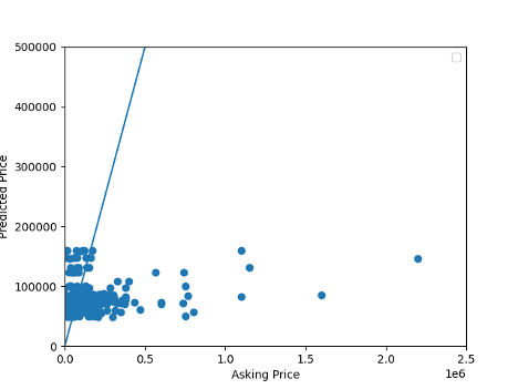
The model was not very accurate. The MSE is 52257562878.595474. Even though the model wasn’t very accurate, it under and over predicted about the same number of homes. It under predicted 146 and over predicted 162. The houses that the model underpredicted the most were the most expensive houses and the houses that were overpredicted tended to be the least expensive.

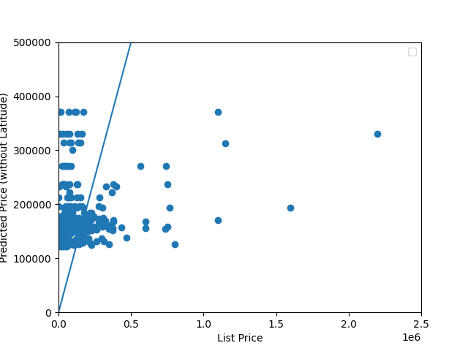
When I ran the model without considering location, the MSE was 48338586251.65768, which is actually better. Perhaps if I had included both longitude and latitude, it would have increased the accuracy of my model instead of making it less accurate.

Figure 2. Listed House Prices compared to Model Predicted House Prices (USD) when model includes latitude. Notice the difference in axis scales.

Points plotted above the line are over predicted, points plotted below the line are underpredicted.

Figure 3. Listed House Prices compared to Model Predicted House Prices (USD) when model has 3 variables (does not consider latitude). Notice the difference in axis scales.

Points plotted above the line are over predicted, points plotted below the line are underpredicted.

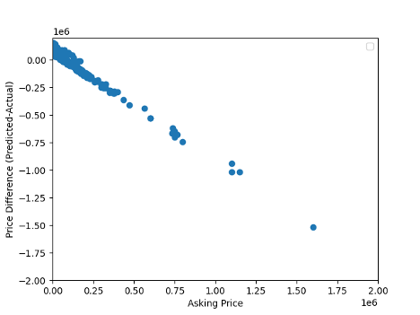
Figure 4. Listed House Prices compared to Difference in price vs. predicted. Notice the difference in axis scales.

Houses plotted below zero are underpredicted and thus are a bad value for the home owners. Houses plotted above zero are over predicted and would be good value for home owners. The graph is pretty hard to read because some of the most expensive houses were so under predicted.

Best Values for current Homeowners: Homes that were over predicted

Worst Values for current Homeowners: Homes that were under predicted